Evaluate and manipulate vcf files
Extract the SNP data as a variant call format (vcf) file with populations from STACKS:
cd ~/RADlecture/stacks
populations -P ./ -b 1 -M ../indmap --max_obs_het 0.65 --vcf
We filter out any loci with more than 65% heterozygote individuals as they may represent pooled paralogs. The result can be found at ~/RADlecture/stacks/batch_1.vcf.
We can use vcftools to produce some basic statistics, like:
vcftools --vcf ./batch_1.vcf --missing-indv
This will calculate the missingness on a per-individual basis. The output will carry a suffix .imiss.
- How much missingness is there present in our raw data?
- Which samples have the highest level of missing data?
Let’s try to remove the sites with missing data. Use vcftools with the option --max-missing which can take values from 0 to 1, where 1 means no missing data allowed. We can also filter by the minor allele frequency (asking to be present in at least 2 individuals):
vcftools --vcf ./batch_1.vcf --maf 0.03 --max-missing 0.8 --recode --out 20miss
Let’s look at the coverage of the data. To calculate the average coverage (depth) per individual:
vcftools --vcf ./20miss.recode.vcf --depth --out 20miss_depth
Open the resulting file with libre office calculator.
We can also inspect further the data. For example we could estimate an inbreeding coefficient:
vcftools --vcf ./20miss.recode.vcf --het --out 20miss_het
- The last command will calculate a measure of heterozygosity on a per-individual basis. An inbreeding coefficient F will also be estimated for each individual using a method of moments. The output will have the suffix .het. Is there a difference in inbreeding between the two ecotypes?
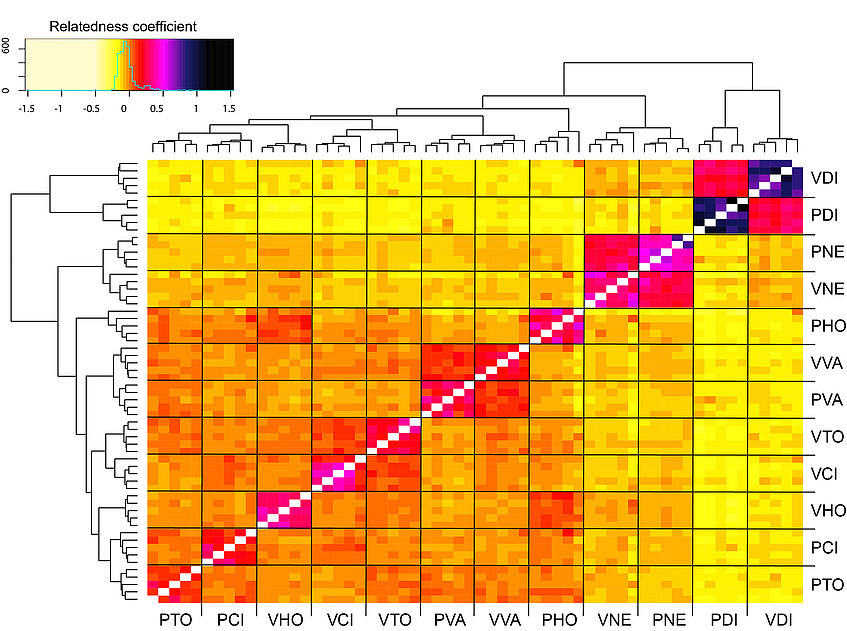
We can calculate also pairwise relatedness estimates between individuals based on the unadjusted Ajk method of Yang et al, Nature Genetics 2010 (doi:10.1038/ng.608) that we can plot later as a coancestry heatmap. Expectation of Ajk is zero for individuals within a populations, and around one for an individual with themselves:
vcftools --vcf ./20miss.recode.vcf --relatedness --out ajk
An overview for different vcftools settings you can find here.
To plot the different measures with R start Rstudio with
rstudio
Then download the prepared Ajk relatedness matrix, the individual definition, and a reformatted sumstats output of Stacks in the RADlecture folder. Set the working directory in rstudio to RADlecture and then load the two datasets:

setwd("~/RADlecture/")
relat <- as.matrix(read.table("ajk"))
sumstats <- as.matrix(read.table("sumstats", header=T))
individuals <- read.table("ind")
ind <- paste0(individuals[,1])
Install and load the required libraries:
install.packages("beanplot")
install.packages("gplots")
library(beanplot)
library(gplots)

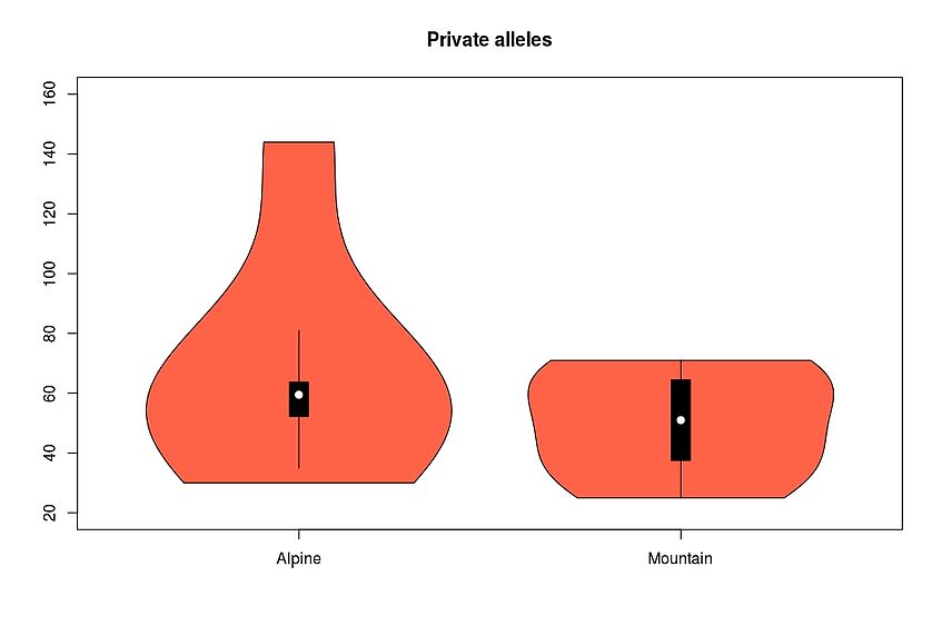
Plot for example the Private alleles as violin plots:
pdf(file = "~/RADlecture/private.pdf", width = 4, height = 4)
beanplot(as.numeric(sumstats[1:6,2]), as.numeric(sumstats[7:12,2]), names=c("Alpine", "Montane"), col=c("indianred"))
title("Private alleles")
dev.off()
Test if the distributions are significantly different:
wilcox.test(as.numeric(sumstats[1:6,2]), as.numeric(sumstats[7:12,2]), paired=TRUE)
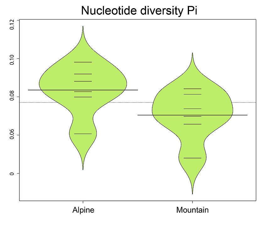
Do the same for other statistics, for example for Observed heterozygosity, Nucleotide diversity, and Inbreeding coefficients.Try also the inbreeding coefficient F calculated per individual with vcftools.
Plot a coancestry heatmap to visualize patterns of relatedness:
pdf(file = "~/RADlecture/heatmap.pdf", width = 4, height = 4)
heatmap.2(relat, trace="none", Rowv=NA, Colv=NA, cexRow=0.6,cexCol = 0.6, labRow = ind, labCol = ind, col= colorRampPalette(c("lemonchiffon", "lemonchiffon", "lemonchiffon", "yellow", "red", "magenta", "midnightblue", "black"))(70))
dev.off()

