Differential gene expression analyses
DESeq2 is a Bioconductor package in R, designed to test RNAseq count data for significant differential expression, making use of biological replication, and normalizing count data on a negative binomial distribution. We start with a count table. To run R you just need to type the following in the command line of a terminal:
R
Then close R by typing (commands that will be typed in R are shown with the specific cursor >, but this does not have to be typed):
> q()
To load the DESeq2 package, start R and enter:
> library(DESeq2)
If you need to install DESeq2 in your R instance use:
> if (!require("BiocManager", quietly = TRUE))
install.packages("BiocManager")
> BiocManager::install("DESeq2")
As input, DESeq2 expects count data as obtained, e. g., from RNAseq, in the form of a matrix of integer values. The value in the ith row and the jth column of the matrix tells how many reads have been mapped to gene i in sample j.
The count values must be raw counts of sequencing reads (ideally uniquely mapping reads). This is important for DESeq2's statistical model to hold, as only the actual counts allow assessing the measurement precision correctly. Hence, please do not supply other quantities, such as (rounded) normalized counts, or counts of covered base pairs - this will only lead to nonsensical results.
Construct the DESeqDataSet object. For this we should provide a matrix of Read Counts, the information for the columns as a data.frame, and a design formula (indicated by ~).
Navigate to your working directory in which you have the table of counts:
> getwd()
> setwd("~/students/YourName/LocX")
> data <- as.matrix(read.table("Xcounts.txt", header=T, row.names=1))
This example is given for locality 1. Please modify accordingly for other localities.
> head(data, 1)
> samples <- data.frame(row.names=c("A1a", "A1c", "A1d", "M1a", "M1c", "M1d"), condition= as.factor(c(rep ("alpine",3), rep("montane",3))))
> samples
The class used by DESeq2 to store the read counts is DESeqDataSet that facilitates preparation steps and also downstream exploration of results. A DESeqDataSet object must have an associated design formula. The design formula expresses the variables which will be used in modelling. The formula should be a tilde (~) followed by the variables. An intercept is included, representing the base mean of counts. The design can be changed later, however then all differential analysis steps should be repeated, as the design formula is used to estimate the dispersions and to estimate the log2 fold changes of the model.
> dds <- DESeqDataSetFromMatrix(countData=data, colData=samples, design=~condition)
> dds
It is important to supply levels (otherwise the levels are chosen in alphabetical order) and to put the putative ancestral "alpine" level as the first element ("base level"), so that the log2 fold changes produced by default will be the expected comparison against the base level.
An R function for easily changing the base level is relevel. An example of setting the base level of a factor with relevel is:
> dds$condition <- relevel(dds$condition, "alpine")
The standard differential expression analysis steps are wrapped into a single function, DESeq. Results tables are generated using the function results, which extracts a results table with log2 fold changes, p values and FDR adjusted p values. With no arguments to results, the results will be for the last variable in the design formula, and if this is a factor, the comparison will be the last level of this variable over the first level.
> dds <- DESeq(dds)
> res <- results(dds)
> head(res)
The lfcSe is standard error value, whereas the stat gives the Wald statistic (i.e., the log2FC divided by lfcSE), which is then compared to a standard Normal distribution to generate a two-tailed pvalue.
We can order our results table by the adjusted p-value and, respectively, make a table including a internal threshold of padj < 0.05:
> resOrdered <- res[order(res$padj),]
> head(resOrdered)
> res05 <- res[which(res$padj < 0.05), ]
- What is the lowest p-value and the corresponding padj? How many genes have padj < 0.05? What about 0.001?
- What is the maximum and minimum log2FoldChange between the two ecotypes? Why are both positive and negative values of log2FoldChange?
- Compare the results between different regions/localities. Can you think why there are differences and how can this be interpreted?
For example to find out the lowest log2FoldChange:
> min(res$log2FoldChange, na.rm=T)
We can get a summary on the p-adjusted values:
> summary(res05)
To check how many transcripts are DE at a level of padjusted < 0.001:
> sum(res05$padj < 0.001, na.rm=TRUE)
We can check the sizeFactor used in the log calculations and save the results table:
> colData(dds)
> res05_Ord <- subset(resOrdered, padj < 0.05)
> write.table(res05_Ord, file = "DESeq2Res05Loc1.txt")
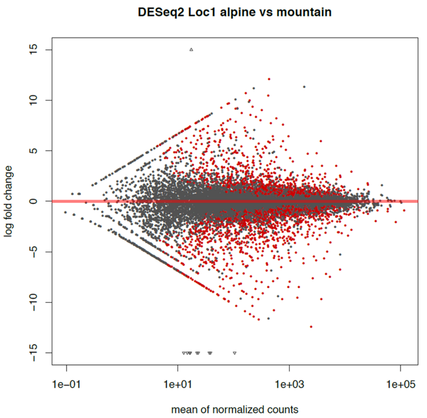
Further, let’s draw an MA plot (if the plot does not look good extend ylim):
> pdf("MA.pdf", width = 8, height = 8)
> plotMA(res, main="Loc1 DESeq2 alpine vs mountain", ylim =c(-15,15))
> dev.off()
This will save the MA plot in a Rplots.pdf file. To visualize the file we will need to download it with scp in a different terminal.
> scp student@vetlinux03.local:/home/student/students/YourName/LocX/MA.pdf ./