Mapping RNAseq reads
Mapping RNAseq reads should be performed with a dedicated, splice-aware aligner, such as STAR. This is an ultrafast RNAseq aligner that outperforms many other mappers. It uses a sequential maximum mappable seed search in uncompressed suffix arrays followed by seed clustering and a stitching procedure. In addition to unbiased de novo detection of canonical splice junctions (i.e., flanked by GU-AG that make up to 99% of splice sites in most organisms) STAR can discover non-canonical splice sites and chimeric (fusion) transcripts.
Normally, it is recommended to use a reference that has already annotated splice junctions or a 2-phase mapping approach with STAR. In the latter approach, in the 1st pass STAR mapping of every sample, de novo information on the intron-exon (reference genome) and exon-exon (reference transcriptome) junctions is being collected and used to generate a new genome index for the 2nd pass mapping. We are going to use the first approach where splice junctions are already available in an annotation file, in .gff format.
First we need to prepare the reference genome for alignment by generating genome index files from the .fasta file (and .gtf or .gff annotation files if available). We will use a subset of 548 contigs (a total of 75,170,146 bp) from the reference genome of Heliosperma pusillum v.1.0 (Szukala et al. 2023). Each contig may contain several genes.
cd ~/students/YourName/Mapping/
nice -n 19 STAR --runMode genomeGenerate --genomeSAindexNbases 12 --genomeChrBinNbits 17 --genomeDir ./ --genomeFastaFiles ./refgenome.subset.fasta --runThreadN 4 --sjdbGTFfile ./refgenome.subset.gff --sjdbGTFtagExonParentTranscript Parent --sjdbOverhang 99
For small genomes/transcriptomes --genomeSAindexNbases (a pre-indexing setting) must be scaled to min(14, log2(Genome length)/2-1). The size of the bins for genome storage (--genomeChrBinNBits) needs to be also scaled to min(18, log2(GenomeLength/NoReferences)). The setting –sjdbGTFfile gives the path to a GTF/GFF file with annotations, including splice junctions. Finally, --sjdbOverhang should be set to maximum read length -1.
In the next step we align the reads of each sample one by one to the reference genome. Here .fasta or .fastq files can be used, but they should be quality trimmed/filtered. To exemplify the step, we will map single end reads from just one individual - the reads have been already trimmed with trimmomatic.
STAR will write several output files, including alignments in .sam or .bam format, mapping summary statistics (a file ending in Log.final.out), splice junctions (a file ending with SJ.out.tab), unmapped reads, etc. There are many options that can be used, here we specify the most important ones.
nice -n 19 STAR --genomeDir ./ --readFilesIn ./A1c.small.fq --outSAMtype BAM SortedByCoordinate --outFileNamePrefix ./A1c --outFilterMismatchNoverLmax 0.1 --runThreadN 4
The options explained:
--runThreadN: number of threads
--outFilterMismatchNoverLmax: report a mapping only if the ratio of mismatches to mapped length is less or equal to this value. Several other filtering values are available.
Examine mapping results
Let’s evaluate the mapping results. To have a look at the summary mapping statistics that STAR produces type
cat A1cLog.final.out
- How many reads did we attempt to align? What is the percentage of mapping reads in this case? What is the percentage of multiple mapping reads?
- Compare the results of the different groups. Are they the same?
We can visualize the .bam file with samtools. After typing the command the entire .bam file will be displayed on screen. Stop the displaying at some point by typing CTRL+C or pipe the command to head. In the VetGrid:
samtools view A1cAligned.sortedByCoord.out.bam | head
The first column in the .bam file gives the read name, the third column gives the contig name on which the read is mapping, the fifth column is the mapping quality which for uniquely mapping reads is by default 255. The field NH:i should also carry a value of 1 for uniquely mapping reads. The rest of the field give the coordinates for the mapping, the number of mismatches, and any splice junctions.
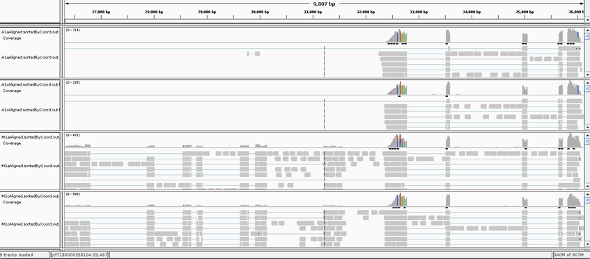
We could also visualize the mapping for example with IGV, but this does NOT work in the vetgrid cluster, so it will be only demonstrated by me. First the mapping file must be sorted and indexed, but this is already done here. After launching the IGV browser, we load the .fasta reference genome with Genomes _ Load Genome from File. Then we load for example A1a, A1c, M1a and M1c (sorted and indexed) .bam mapping files File _ Load from File (i.e., use the strg/ctrl taste to select multiple files).
- Navigate through some of the contigs in the reference, for example go to jcf7180000358104 and select the region ca 27,000bp to 36,000bp. Can you explain the heterogeneity of the coverage?
- Can you identify some mapping outside exons? Is this suprising for this RNAseq data?